It is common practice to perform fits to raw profile data prior to inputting them to TRANSP. This is because TRANSP takes spatial derivatives of some signals in order to solve the particle and heat balance equations and consequently noisy data can lead to large fluctuations in these gradients which then affect the transport coefficients which are derived. Often the use of raw data results in TRANSP crashing. For JET analyses, LIDAR electron density and temperature measurements can usually be used in their raw form, which is implemented in BEAST. There are two ways of producing fitted input profiles - first and most commonly used is a program called Profile Maker, written by A. Baciero, which can be used to perform fits and save the results to private PPFs which can then be read into TRANSP. The second option is OMFIT's native OMFITprofiles module, which is available for use with JET data, but is still being tested. A video tutorial on the use of OMFITprofiles can be found on this repository.
To run Profile Maker log on to the Heimdall cluster and click the 'Applications' button in the desktop toolbar, followed by 'Fusion' and 'JET Analysis Codes', and find the 'Profile Maker' entry.
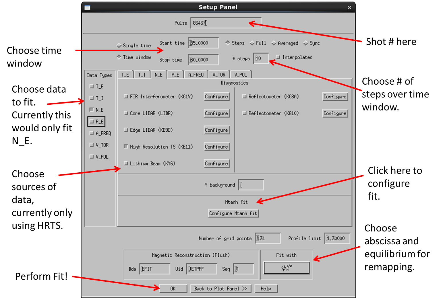
This will open a pair of windows, a setup window and the profile maker plot window. The setup window is shown on the right and allows the user to configure which
data will be fitted. The shot number of interest is entered at the top of the window in the Pulse field. Beneath this is a window which allows the user to configure which
timeslices will be fitted. A single time or a window can be chosen. If a window is specified the user must also specify in the '# steps' field how many equally spaced
timeslices will be fitted in the chosen window. For example if the fits are based on HRTS data, which has a measurement frequency of around 20 Hz, then 20 slices would be chosen per
second of fitting window. The main part of the window allows the user to choose which data sets will be fitted. The bar on the left selects which variables will be
fitted and the tabs allow the user to choose which diagnostics will be included in the data set for each variable.
So in the figure on the right only the electron density will be fitted (N_E)
and for this variable only the HRTS data will be used. Multiple diagnostics can be used in performing a single fit if so desired. Additionally, by clicking the 'Configure' button
next to the diagnostics entry, the user can choose the relative weight of the data in the fit or trim it radially through the '(r/a) limits' entry box. The section beneath
this specifies the selected fitting method , which can be changed in the plot window by clicking the 'Tools' tab in the toolbar. The recommended fit functions are MTANH
when dealing with H-mode profiles with a pedestal, or Cubic spline fit (setting for Tension ~ 5.0e-5) for profiles of L-mode plasmas. Pressing the Configure MTANH fit
button allows configuration of the way this fit is performed,
this usually involves choice of boundary conditions or the order of polynomial fits being used. The bottom section specifies which equilibrium is being used to perform variable
transformations. In this case EFIT is being used and the chosen output radial variable is .
Other options include ,
and normalised minor radius. Please note that the
setting of the radial variable in Profile Maker needs to match the setting in OMFIT/TRANSP when reading in the created PPF. Once the configuration is as desired press the
OK button to perform the fits.
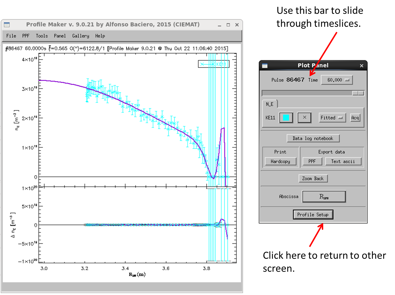
Once the fits are completed the two screens shown left will be visible. The large white panel is the plot window which shows the data and the resulting fit. The second panel
shows which markers correspond to which data sets and allows the user to slide through the different timeslices for which fits have been perfomed. It is highly recommended that
users slide through all individual profile fits and check for any fit deviations. These usually include errors in pedestal fitting or extrapolated core profile gradients. The
manual scanning exercise might sometimes be tedious, but the effort is reflected in the quality of the TRANSP simulation result. To return to the setup window
click the large Profile Setup button at the bottom. To save a PPF of the fit results click on the PPF button underneath the Export Data label.
The pop-up window enables you to select the fits and timeslices you wish to be written out, and thus filter out any unsuccessful fits. Choose a DDA name for the PPF and then click
Write PPF. The resulting PPF profiles are read into TRANSP through OMFIT in the third step of the run preparation - Load Profile Ufiles as described in this
google doc - where you need to input
the PPF credentials chosen in Profile Maker.
If you wish to use a different type of fit, the various options can be selected from the drop-down tools menu at the top of the plot panel. In order to use the selection you must return to the plot setup panel and rerun the fitting process.
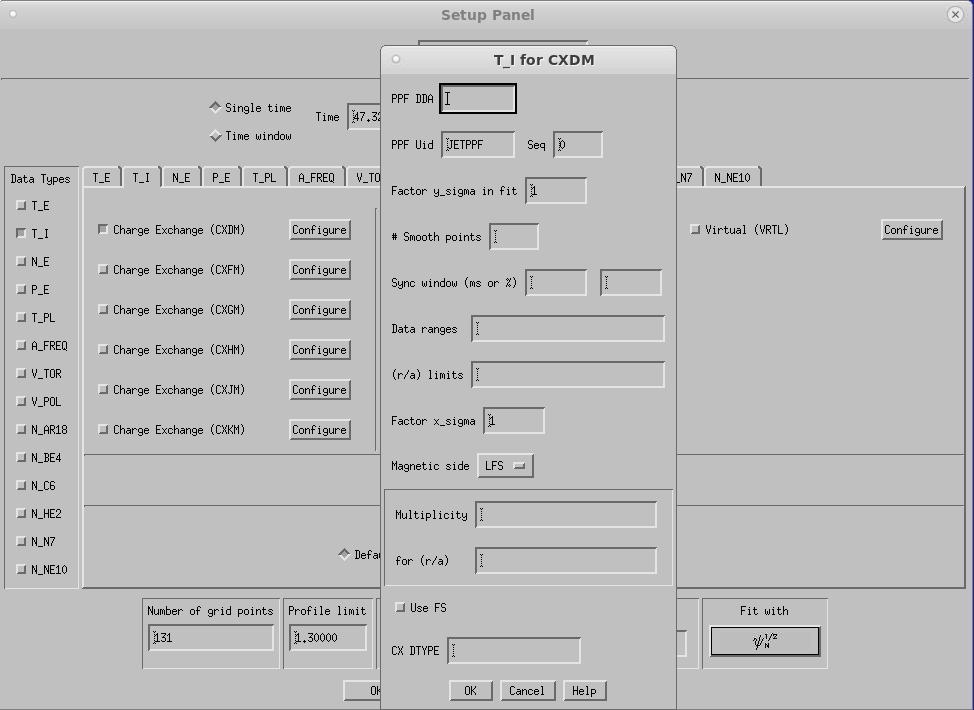
TICR and TIFS are separate corrections aplied to TI datatype. Usually TIFS is a larger correction compared to TICR. It is recommended that a user used consistently one if the chosen datatypes throughout performed analysis.
While choosing Ti DDA's to be used one may configure the ppf details by clicking on Configure button (Left: next to Charge Exchange option). Ti datatype can be chosen in two ways:
'use FS', TIFS datatype will NOT be used if TICR is available. Since some pulses have TICR along with TIFS available and some only TIFS it makes it harder to perform a consistent analysis.
CX DTYPE. Using this option overrides 'use FS' option.
It is advised to use core CX datatypes by explicitly specifying them in the field CX DTYPE.