Under normal circumstances TRANSP is provided with the plasma boundary, the species densities and temperatures, the total plasma current and the edge value of rBTor as inputs. The plasma pressure can be calculated using the input temperatures and densities (see the pressure section below). The plasma q profile is either input directly or calculated via solution of the Poloidal Field Diffusion Equation. It is also usually modified at the edge to match the constraint given by the total plasma current. Using these inputs TRANSP solves for the plasma equilibrium internally using the TEQ equilibrium solver. To determine the equilibrium TEQ numerically solves the Grad-Shafranov equation:
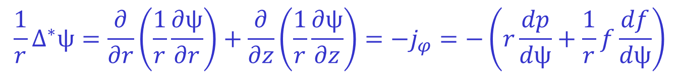
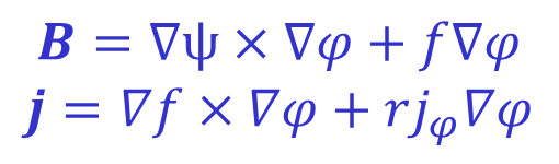
Where ψ and f are the poloidal flux and current functions defined by:
Solution of this equation requires knowledge of the functions p(Ψ) and f(Ψ). Normally f is not input directly, instead it is the value of q which is known. Consequently it is necessary to derive an expression for f in terms of q. The first step towards deriving this expression is to determine a relation between the infinitessimal toroidal angle dφ traversed for a given infinitessimal poloidal path length dl when following a magnetic field line around the plasma:
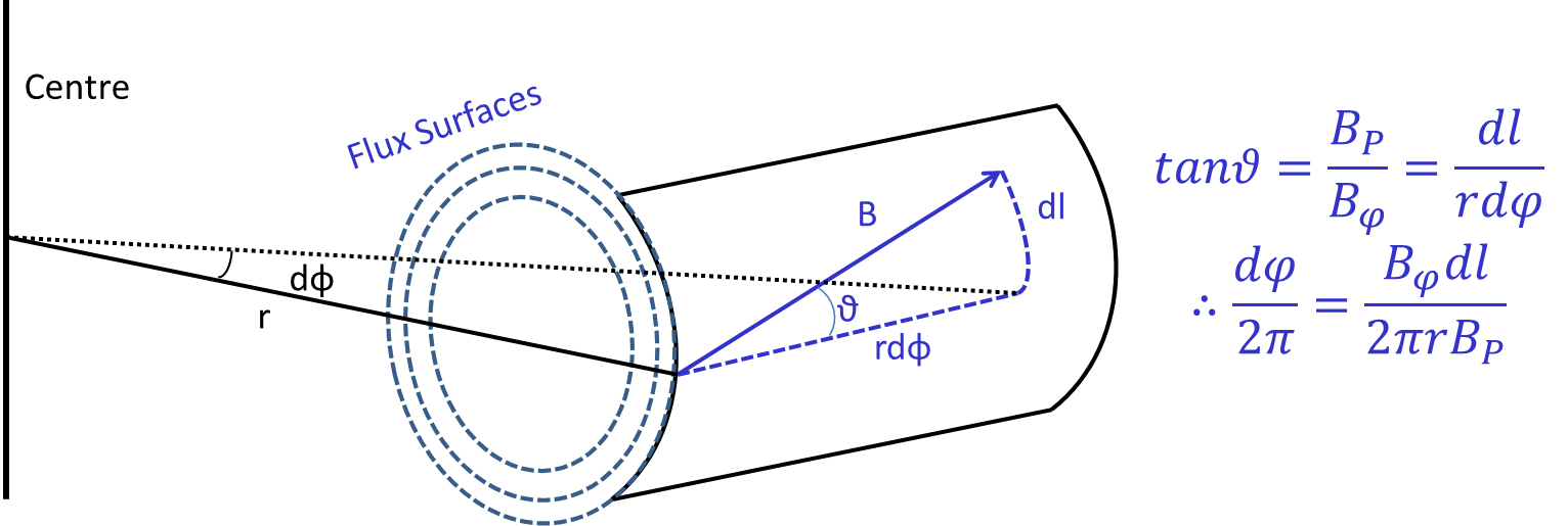
Then, using the fact that q is defined as the number of toroidal turns per poloidal turn, one can calculate q by finding the toroidal angle subtended when following the B field once round poloidally.

Where L indicates a closed poloidal contour. Moving from the first to the second integral exploits the relation derived above for the toroidal angle traversed when following the B field while moving from the third to the fourth uses the fact that f=rBφ as can be seen from the expression for the magnetic field given above. The last step converts from a line integral around a poloidal contour to a surface integral over the flux surface S by dividing by 2π and exploiting the fact that BP=|∇ψ|.
A simpler way of expressing this relationship can be found by utilising the definition of the flux surface average. This is in fact a volume average over an infinitessimal volume between adjacent flux surfaces. It is defined as follows:
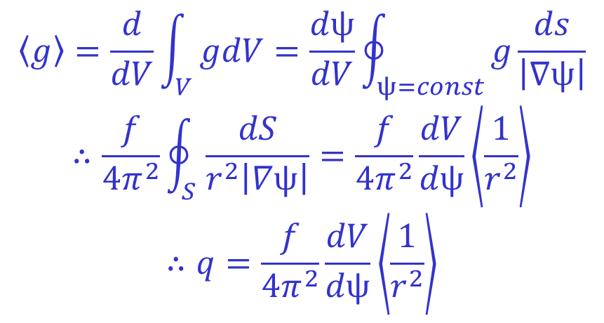
Note that this relation relies on a priori knowledge of the flux surfaces in order to calculate the surface average of 1/r2. Consequently this equation for f(Ψ) in terms of q(Ψ), input profiles of q(Ψ) and p(Ψ), and the Grad-Shafranov equation constitute an implicit system which can be numerically solved for the equilibrium.
TEQ does not normally iteratively solve for a consistent equilibrium but instead uses the equilibrium from the previous time step to calculate the relationship between q and f and to map any input radial data from major radius (for instance) onto Ψ. To initialise the equilibrium solver a 'fake' equilibrium is used which is based on a moment representation which matches the plasma boundary and has the correct asymptotic behaviour as the axis is approached. This is used to map radial data onto Ψ, calculate f(Ψ) and solve the GS equation to produce a new equilibrium. This is repeated 5 times prior to beginning the time stepping in order to converge to a reasonable initial equilibrium. The numerical techniques which TEQ uses to solve the Grad-Shafronov equation given p(Ψ) and f(Ψ) are based on the techniques described in this paper which provided the source material for this section.
The pressure used by the equilibrium solver is a sum of several components:
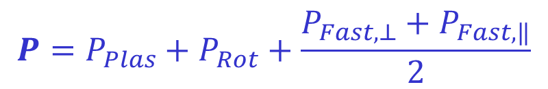
Where PPlas is the sum of the thermal pressures of the electrons and ions, calculated using their known temperatures and densities, PRot is
given by 4/3 of the rotation energy density and the perpendicular and parallel fast ion pressures are determined using the corresponding energy densities calculated by NUBEAM.
This pressure is stored as an output signal named PTOWB. Prior to being handed to the equilibrium solver this pressure may be further modified based on selected
namelist settings and will then be smoothed. The final pressure which is handed to the equilibrium solver is stored in the output variable PMHD_SM.