TRANSP is a 1.5D interpretative plasma transport code originally developed at Princeton Plasma Physics Laboratory. What this means practically is that TRANSP uses a set of diagnostic input data augmented with models for quantities which cannot be easily measured to solve the particle and energy balance equations. In doing so TRANSP allows a determination of the transport coefficients during a particular shot as well as a huge amount of supplementary information which can be valuable in building a coherent picture of the evolution of a plasma and an understanding of the transport processes occuring within it. The '1.5D' part means that while TRANSP deals with a full 2 dimensional magnetic equilibrium, the quantities of interest are considered constant over nested toroidal flux surfaces and hence can be considered 1 dimensional functions of an appropriately chosen radial variable. In TRANSP the radial variable chosen is , the square root of the toroidal magnetic flux normalised by its value at the plasma boundary.
This page gives a basic overview of the execution of TRANSP as it is commonly run at JET. It is important to remember however that TRANSP is highly configurable and that many of the settings and modules decribed below can be changed and that ultimately what is done will depend on the availability and quality of experimental data. For more information on this see the namelist section. The discussion is a modified version of the summary given in this paper by J.P.H.E. Ongena et al. A more thorough exposition of the basic equations being solved by TRANSP is given in this paper by B. Grierson. Extensive documentation on models and input switches can be found on the TRANSP help webpages.
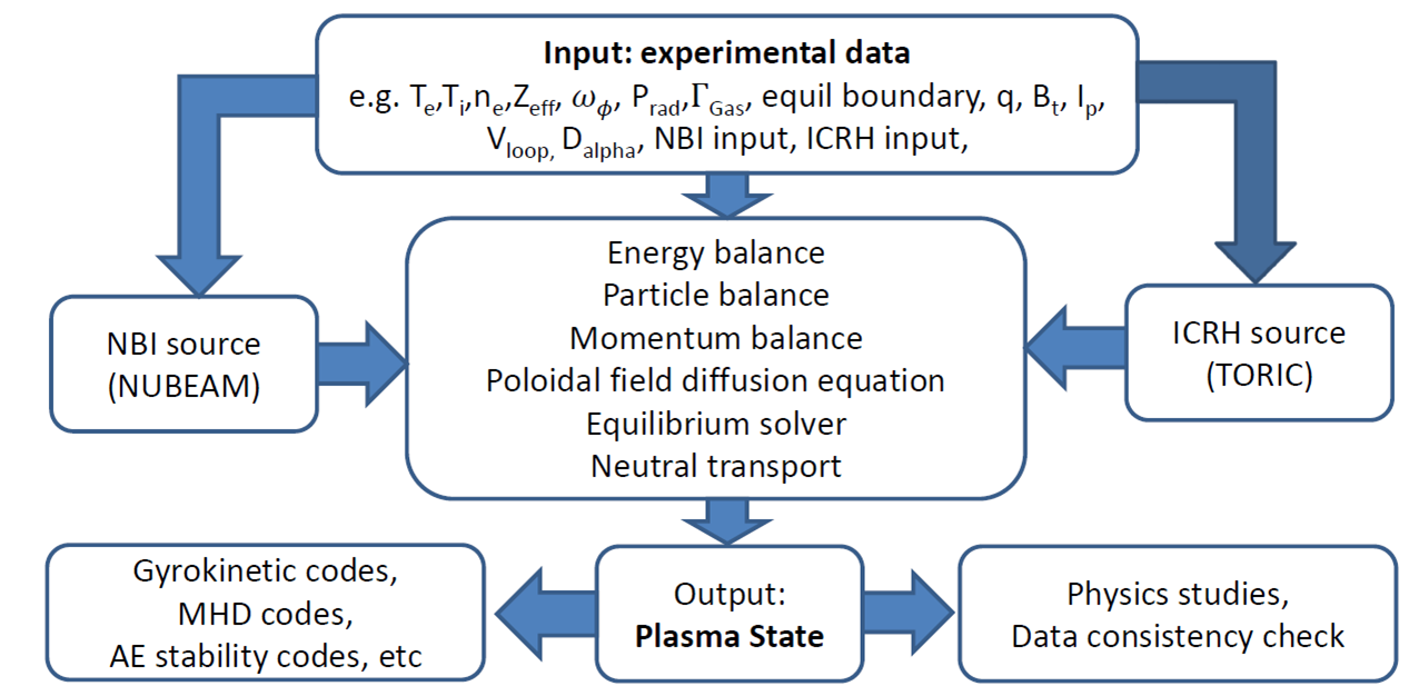
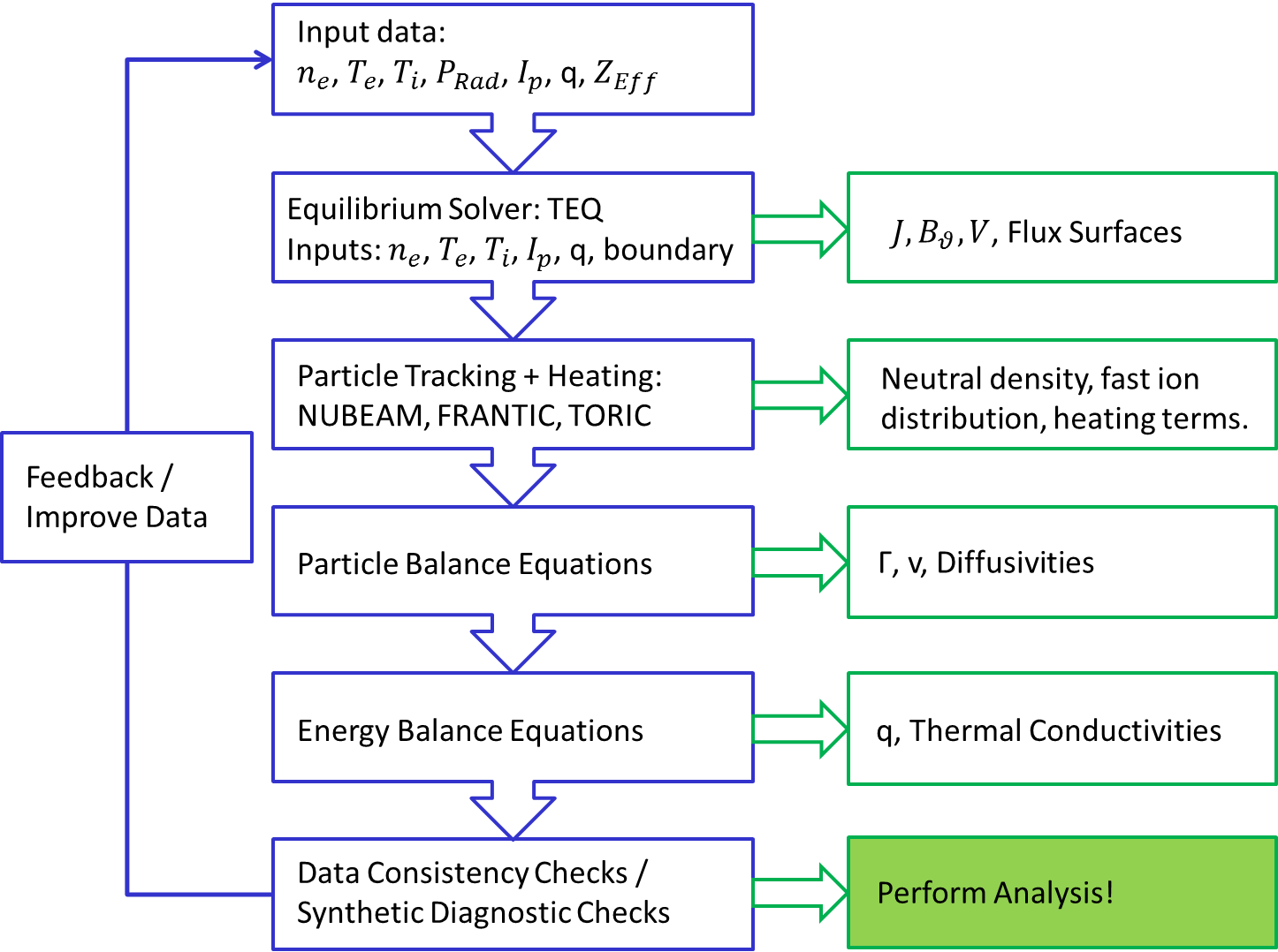
A typical input data set to TRANSP at JET might be the following:
Note that the ion density is not specified. The density of thermal ions and impurities can be determined using the electron density, quasi-neutrality and the input value of .
The first step TRANSP takes is to solve the Grad-Shafranov equation to determine the equilibrium configuration for the plasma for the current time step. In normal usage a module called TEQ is called which solves the Grad-Shafranov equation using the input q profile, plasma boundary, plasma current and pressure as constraints. For more information on this, see the page on TEQ. Once TEQ has run, the nested toroidal flux contours are known, as are the magnetic field and current profiles. If the measured surface loop voltage has been input this can be compared with the calculated value as a consistency check on the determined equilibrium. The transport equations are then solved by dividing the poloidal cross section of the plasma into a discrete set of zones between flux surfaces and performing flux surface averages over these zones.
Ultimately TRANSP solves the electron and ion energy balance equations. In order to do this it needs to know the radial velocity profiles v of the electrons and ions and these are currently not known. To determine these the particle balance equations are solved first:
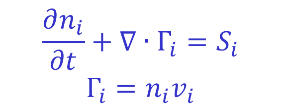
In the above equation i is a species label which can be electron, ion or an impurity species. The densities of the species are known from the input data as described above. The term S represents sources and sinks of particles which must be calculated. These can be split into volumetric sources and sources due to the flux of neutrals from the wall. In order to calculate the sources of particles TRANSP utilises dedicated fast particle and neutral penetration codes. The fast particle tracking code is named NUBEAM and models both the neutral beams injected into the plasma, their subsequent ionisation by processes such as collisional ionisation and charge exchange, and then the evolution of the resulting fast particle distribution. In order to do this NUBEAM must know the geometry of the neutral beams being used, the fractions of power in the different energy states in the beam and the total power being supplied by each PINI. When TRANSP is run at JET this information is acquired automatically by OMFIT, the geometry information is stored in the TRANSP namelist file while the input power signals are written to a file. The distribution of neutrals is tracked by a neutral penetration code named FRANTIC. These two code interact with each other as charge exchange and ionisation processes are sources and sinks of both the neutral population and the fast ion population.
Having solved the particle balance equations for the different species to determine the radial flow velocities one can now consider the energy balance equations:

The left hand sides of both equations contain in order terms describing: the rate of change of energy of that species, the heat flux loss for that species, energy losses by convection for that species and lastly work done by the plasma against a pressure gradient. The right hand side terms represent the various sources and sinks of energy for the different species.
The ion energy balance equation is considered first. The terms on the right hand side in this equation represent: auxillary heating from neutral beams and RF heating, this is calculated by the NUBEAM fast particle following code and by the TORIC RF heating code; the energy gained from ionisation of neutral particles by electrons, which is given by where is the neutral temperature; the energy gained by the ions via collisions with the electrons given by
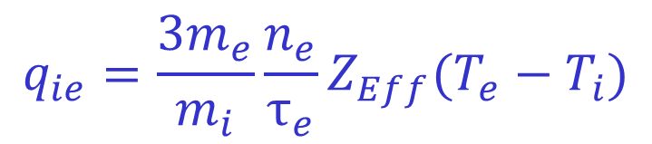 ;
;
and lastly energy lost via charge exchange interactions, which is given by . If, as in our example, the ion temperature profile is known, this equation can be solved for the ion heat flux and consequently the ion thermal conductivity:
If it is not known, perhaps because charge exchange information is unavailable, the ion temperature can be deduced from this equation by setting the conductivity equal to its neoclassical value (or the value derived from any other transport model). It is however more common when performing interpretative simulations to set the ion temperature equal to the electron temperature in this case.
Lastly the electron energy balance equation is solved to determine the electron thermal conductivity profile. The terms on the left hand side of this equation are equivalent to those on the left hand side of the ion energy balance equation. The terms on the right hand side represent: The ohmic heating, which is calculated from the current profile as ; The auxillary heating to the electrons from beam injection and RF heating, again calculated using NUBEAM and TORIC; the energy loss to the electrons from ionising collisions with neutrals, given by where is the energy loss from an ionising collision; the energy lost by bulk radiation from the plasma, this is input data obtained from bolometry measurements and lastly the energy lost via collisions with the ions.
This is the basic set of steps TRANSP makes for each timestep of the simulation. Note that none of the input data is being 'evolved' through time, the equations are just being solved for their unknowns at each timestep. If only the initial q profile is known then it is possible to evolve this through time by solving the Poloidal Field Diffusion Equation however usually the q profile is specified and so this is not required. Lastly it is important to remember that while the end point of these calculations was a determination of the thermal conductivities and particle diffusivities of the different species, many auxillary quantities are calculated in the process including current and field profiles, heating profiles, momentum and heat fluxes etc. This provides a wealth of information with which to analyse a particular shot. An outline of the steps taken and the outputs they produce for our example is shown below.